Searching for a specific value among a set of unsorted values is quite easily solvable, even to those new to computer science: add the values to a well-defined data structure, sort, and execute a search algorithm. Collectively, this has a time complexity of O(nlog(n)). When the target value is unknown beforehand, the problem becomes more difficult.

This type of searching is distinct from the classical sort-and-search problems, in that the value we seek is unknown, and therefore its position or relation to the space in which it is defined is likewise unknown. This class of problem is broadly known as Search-and-Rescue, and is somewhat related to distributing computing problems in terms of analysis. The rescue portion of these problems factor in the cost of returning to the starting point after a successful search, which is trivial; it is the searching algorithm that is the focus.

Linear (1D) Search

We may begin with a formal definition of the problem.

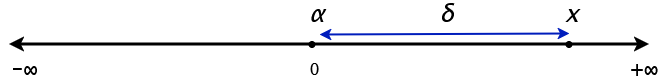
A mobile agent α begins at the origin 0 of a line. The line is infinitely long in both the positive and negative directions. For simplicity and illustrative purposes, let the negative direction be referred to as the left, and the positive direction be referred to as the right. The agent α is capable of moving at a speed of 1. An object x lies at some point along this line distance d away from the origin. x is strictly not at the origin is placed randomly. What algorithm should α follow to locate x and how efficient is it in comparison to an algorithm with perfect knowledge?

This is quite a straightforward question and only requires a bit of math and thinking, but I love it because accurately describing its efficiency involves the concepts of the competitive ratio and the adversary. I will define them briefly before continuing with the problem.

The competitive ratio of an algorithm A’ is the ratio of the time or some other cost required by A’ to complete and the time or cost required by the optimum algorithm A with perfect knowledge. Naturally this ratio is either 1 or greater as it is logically not possible for an algorithm to perform better than the best-performing algorithm.

The adversary is a hypothetical actor or environment that works against the algorithm such that it guarantees the worst case scenario. Just as Big-O notation refers to the worst-case time complexity, the adversary ensures an algorithm A’ spends the worst-case cost. The competitive ratio uses the adversary to refer to the worst-case ratio. The term adversary connotes an actual actor, but this is all hypothetical. The adversary concept simply means that when calculating the competitive ratio of A’, we analyze the worst case scenario as specifically designed to work against A’.

Let’s begin by formulating A’ for the linear search problem, but with an advantage: A’ knows whether x lies to the left or the right of the origin. What should A’ be and what is the competitive ratio? A’ already knows which direction x lies in, so all A’ should logically be is

 - travel in the direction of x at speed 1 until x is reached

Since α moves at speed 1, and travels d distance, we can say that that α has taken d time. This is also the same time taken as the optimal algorithm which knows both the direction and the distance d (although d is redundant given the direction). So, quite intuitively, if the direction of x from the origin is known, we can implement an algorithm with a competitive ratio of d/d which is 1.

What about if the direction is not known, but d is known? In this case we simply pick a direction and travel for d distance. If we’re lucky, we’ll find x and terminate. If x is not found, then we change the direction and travel 2d, at which point we find x. Our algorithm would be

 - select a direction
 - travel d distance in the given direction at speed 1
 - if x is not found, change direction and travel 2d distance at speed 1

If we initially select the correct direction, we proceed directly to x and the time taken is as the previous case: simply d. But if our guess is incorrect, then α travels a distance of 3d, comprising of 1d in the initial direction, 1d in the opposite direction to return to the origin, and another 1d to reach x totalling 3d. Since x is placed either to the left or right at equal probability, this means half the time our algorithm guesses correctly and performs optimally costing d. The other half of the time, it guesses incorrectly costing 3d. It follows that we may expect our algorithms cost to be 2d, or twice that of the optimal algorithm…right?

Maybe, but this goes against how we described our conditions for analysis. The adversary guarantees the worst case for our algorithm; one can almost describe it as first seeing the direction guess, followed by placing x in the opposite direction, such as to ensure the first guess is always incorrect. This of course means our cost is 3d and the competitive ratio is 3.

Our final case of single-agent linear search is when we do not know d or the direction of x. Our algorithm must again search in both directions. When should the mobile agent decide to search to the left or right?

The agent will have to alternate between searching to the left and right in a specified pattern. We can divide the algorithm into rounds. Each round covers a larger distance than in the previous rounds.

Suppose our agent begins at round 1. It first travels to the right a distance of 1. It then returns to the origin and travels to the left a distance of 1 before returning to the origin again. Every k-th round, this is repeated but for a distance of k. Can we compute competitive ratio of this algorithm? First, we must determine where the adversary will place x. Since our robot begins each round by traversing to the right, the adversary places x somewhere to the left. On round k, a distance of 4k is traversed, assuming that x is not found on that round. The adversary places this at the minimal value just beyond a value of k such that α does not reach x on round k, but wastes time in round k + 1. For example, the agent places x at 9.01 (or some other infinitesmally small factor), such that on round 9 α barely misses finding x and instead finds x on round 10 (k + 1). The adversary does not place it the farthest distance possible, but rather the position that makes A’ the most inefficient compared to the optimal algorithm.

Unfortunately, this algorithm is highly inefficient and we want to be able to compute hard limit on the competitive ratio. The agent spends excessive time traversing distances it has already covered.

Let’s propose a different algorithm to address these two drawbacks. Our algorithm should increasingly cover more distance as it changes direction by and increasingly large factor; increasing it by 1, corresponding to the round number, is far too inefficient. We’ll change this to increase the distance exponentially by doubling it each round. The round number will act as our exponent. We begin at round index 0 and selecting a direction at random. We travel a distance of 2^r in that direction and return to the origin. Then we switch directions and set r = 2^r, repeating until x is found.

Of course, the adversary will act similarly as in the previous algorithms. The adversary placed x such that our robot will barely miss it on round k, where it travels a distance of 2^k. It then returns to the origin and wastes another 2 * 2^(k + 1) distance tavelling in the other direction on the next round. On round k + 2 it then travels d distance and finds x.

d of course is not known exactly. But we know its displacement from the origin to be between 2^k and 2^k + 3, since it is guaranteed to not be found on round k and guaranteed to be found on round k + 2. Deceptively similar to our previous algorithm, but it turns out to be very convenient. The total distance this travels is

 2 * (2^0 + 2^1 + 2^2 ... 2^(k+1)) + d

d is the distance travelled on round k + 2. The multiplication factor of 2 on the previous round is the distance to and from the origin. The terms 2^0 to 2^k can be simplified to 2^(k + 1) - 1, which means we can further simplify the equation to

 2 * (2^(k+2) - 1) + d

This is roughly equivalent to 2^(k + 3) + d as the constant term -1 can be ignored at large values of k. We can separate k and rewrite this as 8 * 2^k + d. We don’t know exactly how k is related to d, but as we stated before, we know 2^k is less than d. If we substitute 2^k for d to get 8 * d + d, we simplify this to 9d, which is an upper limit because we substituted a larger value. Thanks to the adversary, d is likely barely larger than 2^k, so we may assume they are about equal.

Our competitive ratio is 9d / d or 9. This is a hard limit! We now have an algorithm that we can guarantee will travel no more than 9 times the minimum distance to find x. This is in fact the best performance. Any other linear search algorithm in the same set up will perform at best with a competitive ratio of 9.

And that completes our analysis of linear search for this problem setup! If the direction is known, there exists an algorithm with a competitive ratio of 1. If the direction is unkown but the distance is known, we can devise an algorithm with a competitive ratio of 3. And if no information is given, the best ‘offline’ algorithm has a competitive ratio of 9. There are of course different problem setups, including multi-robot linear search with differing communication methods, and it is further complicated by adding an evacuation step.

Linear Search Script

Below is an implementation of this algorithm, which will allow us to verify its correctness in practice. This script mimics a line with a minimum, maximum, and origin value. The position for x is selected at random. The while loop then calculates the distance covered each round, along with the total distance, until the distance covered that round in the direction of x exceeds the displacement of x. This indicates x is found on that round. Dividing the total distance by the minimum distance indicates the efficiency of the algorithm for that position of x.

By doubling the distance covered while alternating between directions, the algorithm is guaranteed to locate x after traversing a distance of at most 9 times the minimum distance.

import random

MAX = 1000000000000000000.0
MIN = 0.0
ORIGIN = 500000000000000000

x_position = random.uniform(MIN, MAX)
x_direction = 1 if x_position >= ORIGIN else 0
opt_dist = abs(x_position - ORIGIN)
direction = random.randint(0, 1)
exponent = total_dist = 0

print(f'X position at {x_position} in direction {x_direction}')

while(True):
    round_distance_covered = 2**(exponent + 1)
    exponent += 1
    direction ^= 1

    if ((round_distance_covered / 2) >= opt_dist and direction == x_direction):
        total_dist += opt_dist
        break

    total_dist += round_distance_covered

print('X has been located.')
print(f'Minimum distance: {opt_dist}')
print(f'Total distance: {total_dist} and a min of {opt_dist}')
print(f'Ratio: {total_dist / opt_dist}')

I wrote this post mostly off the top of my head, but I have decided to include two papers below for further reading, in case I would like to revisit this topic. The paper by Czyzowicz et. al. shows how the rescue (or more aptly named evacuation, since there are multiple searchers) phase adds more complexity to the design of such algorithms. I intend to eventually write a post on that topic, but not before I write about other distributed algorithms, since this is meant to serve as a gentle introduction.

R. Baeza Yates, J. Culberson, and G. Rawlins. Searching in the plane. Information and Computation, 106(2):234-252, 1993.

J. Czyzowicz, E. Kranakis, D. Krizanc, L. Narayanan, J. Opatrny, Search on a Line with Faulty Robots. In Principles of Distributed Computing (PODC) 2016.

The Algorithms and Limits Infinite Linear Search

Linear (1D) Search

Linear Search Script

Related Works